Introduction
I am going to give you my nine top tips for data science. Let me start by telling you some stories.
My love for mathematics started when I was about 14 years old. Unfortunately, I had previously been very bad at it but with my new teacher, Gillian Butler, with whom I stayed for five consecutive years it became a passion. The passion was such that I decided to specialize and in my last two years of school I studied Pure Mathematics, Applied Mathematics, Physics and Computer Science.
Whilst I was at school I had a job working at a bar. The bar manager, cliff, had given me the job because I had said I was good at math. However, I couldn’t do arithmetic and I made mistakes in the bar prices. I tried to explain the difference between math and arithmetic but he couldn’t understand and he thought I was bad at math. Now I feel like Cliff. Many young people tell me about the math that they do and I am the one who doesn’t understand.
Alleyn’s School
Since school I have studied Mathematics at the university of Exeter and have then built a successful company that blends IT and Mathematics to sell consultancy solutions to top companies such as Nokia, Vodafone and Microsoft. A typical project sells for around 300,000 dollars but we have other projects that we work on over a period of years and for which we may receive millions of dollars. But why do we have great success? I believe that at a lot of the new math is actually old math that has been re-branded and the old techniques really do help.
A test of your skills
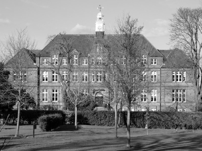
A client has asked us to draw a chart of $f(x) = 2^{-x}sin^2(x^2) x \ge 0$ and I have prepared four possible solutions. But which one is correct? A good data scientist will spot the right one in just a few seconds. This is because the other three have clear defects which immediately rule them out. However, can you spot the rogue charts? This brings us to the first of our top tips for data science.
A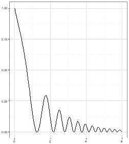 |
B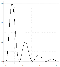 |
C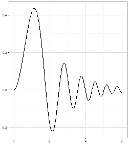 |
D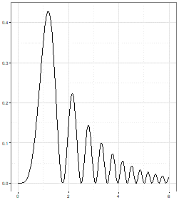 |
Top Tips For Data Science 1
“Query what you are being shown. Don’t accept things at first sight and develop an inquiring eye.”
Top Tips For Data Science 2
“Just because a person in authority tells you something that doesn’t mean that you don’t have to validate what they say and it doesn’t mean you don’t have to challenge them.”
Seeing the problem the easy way
One of my early loves was for seeing a hard problem in a way that makes it look easy. For example, I was fascinated by the simple series formed by adding successive integers.
$S = 1 + 2 + 3 + 4 + \dots + 1000$
This looks easy to calculate manually for a few digits but computing this without error up to 1000 seems hard. But, then I learned a trick. The trick is to write the problem twice:
$S = 1 + 2 + 3 + 4 + \dots + 1000$
$S = 1000 + 999 + 998 + 997 + \dots + 1$
Then we can add the two versions of the equation together to give us:
$2S = 1001 + 1001 + 1001 + 1001\, + \dots + 1001$
Most mathematicians remember the formula $\sum_{i=1}^n i = \frac 1 2n(n+1)$. However, I believe that once you see the trick then you will always be able to derive the formula and the trick is easier to remember.
A story from the battles: Part 1
We were working on a fraud investigation of an African oil company. Documents had been raided from their London offices and there were a lot of word processor files on floppy disc but these had a password. We were asked to try breaking the passwords to be able to read the documents. Instead we bought a copy of the word processor package and wrote our own document and then saved two versions. One without password and one with.
We couldn’t understand the algorithm that was encrypting the passwords but we could see that the encrypted password was always stored in the same place in the file and that the version without a password had zeros in these locations. So, instead of decrypting the passwords we modified the bits and bytes of the protected files to return the password bits to be zero again and we were able to open the protected files. The client thought we were decrypting hundreds of passwords but we didn’t need to decrypt to be able to open the file.
Top Tips 3
“Always try to look for the point of view that gives you the easy answer. Not just in mathematics but in business too. There will often be an easy option if you can just find it. It is always worth looking at the problem from different angles to get the answer.”
Everyone has heard about Pythagoras’ theorem linking the sizes of the three sides of a right angled triangle. It seems difficult but the following picture allows us to explain it to anyone who understand how to compute the area of a square:

This example is extremely elegant and shows how, once again if we find the right point of view then things become easy. Einstein once said if you can’t explain it simply then you don’t understand it well enough.
A story from the battles: Part 2
JTA was asked to help with a project in Paris that had been done, at great cost by a very famous consulting company (it has over 10 billion dollars of worldwide revenue). They had developed a mathematical formula to explain our client’s business that used lots of numerical inputs, such as churn rates, population demographics and so on. It was ingenious but it could not be used as the client had no idea of the values of these numbers.
The consultants had started work without thinking of what was practical to do. Specifically, they did not begin with the end in mind.
We simplified the solution to use data that already existed and we then made things even easier by building a system to calculate the data and the output. JTA still works with this Parisian client today and the top consulting firm were not asked to participate in the project any more. From these stories we can bring out some more of our top tips.
Top Tips For Data Science 4
“Don’t make simple ideas complex. Make complex ideas simple.”
Top Tips For Data Science 5
“Mathematicians can see things from a theoretical view. But, in business we need to be able to implement a solution quickly and reliably. Be both theoretical and practical and you will have great success.”
Seeing the problem the computer’s way
When I was around 15 I met my first computer. It was called an Elliott 903 and it was hand built entirely from transistors because the silicon chip had not been invented.
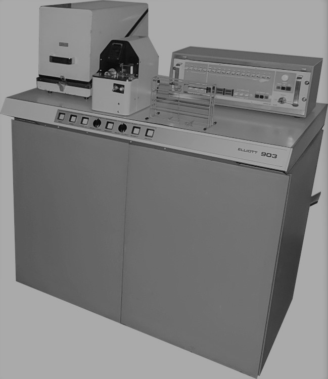
Now there are only a handful of these machines surviving in museums. It had 8,192 words of memory that was formed by small magnetic cores and could perform 16 instructions. Here are the main twelve:
| Data Movement: | Load from memory | Store in memory | Input / Output |
| Basic Math: | Add | Subtract | Logical AND |
| Other Math: | Multiply | Divide | Shift Left or Right |
| Control: | Always Jump | If Accumulator = 0 Then Jump | Jump When Accumulator < 0 |
We could load compilers from paper tape so we could write code in early languages such as Fortran and Algol. As a mathematician I was fascinated by the fact that in our high level language, I could use floating point arithmetic. For example, I could write something like this:
Early Algol
integer j;

real pi;

pi = 3.142

for j := 1 step 1 until 360 do

print sin(j * pi / 180)
Our mechanical teletype would then produce trigonometric values. However, each word in the machine has 18 bits which can hold an integer value from 0 to $(2^{18}-1)$.
So, mathematically speaking, a word holds a limited amount of simple integers $w \in I \quad 0 \le w < 262144$. So, I asked myself:
| Question: | Answer: | |
| 1 | How does the system store negative values? | Use the two’s complement function so the most significant digit becomes the sign bit $ w = \{ \sigma, 2^{17}, 2^{16}, \dots, 2^0 \}$ so we now have $w \in I \quad -2^{17} \leq w < 2^{17} \quad 131072 \leq w < 131072$ |
| 2 | What about fractions? | Consider the digits as $w = \{ \sigma, 2^{-1}, 2^{-2}, \dots, 2^{-17} \}$ not $w = \{ \sigma, 2^{17}, 2^{16}, \dots, 2^0 \}$ so $w \in \R -1 \leq w \leq 1-2^{-17}$ and the smallest non zero value possible is $2^{-17} \approx. 0.000007$. |
| 3 | How does it store numbers requiring more than 5 decimal places? | Use more than one word $w \in \Re \quad w=w_1w_2 \quad w_1= \{ \sigma, 2^{-1}, \dots, 2^{-17}\} \quad w_2 = \{2^{-18}, \dots, 2^{-36}\}$ so $w \in \Re \quad -1 \leq w < (1 – 2^{-35})$ and the smallest non zero value is $2^{-35} \approx 2.91 \times 10^{-11}$ |
| 4 | What about larger numbers like 20 million? | Use a mantissa and exponent $x = m \times 2^e$ where $m$ uses format 3 and $e$ uses format 1. |
It was whilst I was researching these issues that I learned that obvious mathematical “facts” confuse computers.
Mathematicians will say $n+1 \ne n$ but a computer disagrees
| R Console | Explanation |
| n = 1 | We define n to be 1 |
| n+1==n | Let us ask if n+1 is equal to n. Note that in R ‘==’ is used to test equality |
| FALSE | The computer agrees with us that it is clearly false. |
| n=10000000000000000 | We set n to $10^{16}$. |
| n+1==n | The scale of $10^{16}$ and $10^{0}$ is so different the computer can’t sensibly add them. |
| TRUE | So it says that, in its opinion n+1 is equal to n. |
Mathematicians will say $\Big (\sqrt n \Big ) ^ 2 = n$ but a computer disagrees
| R Console | Explanations |
| n=4 | We set n to be 4 |
| sqrt(n)^2==n | We ask the machine if the square of the root is unchanged |
| TRUE | And it is. Note that the square root of 4 is an integer |
| n=11 | The next example is interesting because $\sqrt {11}$ is irrational. |
| sqrt(n)^2==n | So the computer should need $ \infty $ space to store the root. |
| TRUE | But the system agrees with the math and declares TRUE. |
| n=17 | |
| sqrt(n)^2==n | The next example $\sqrt {17}$ is also irrational. |
| TRUE | But the system declares a TRUE. |
| n=13 | |
| sqrt(n)^2==n | The next example $\sqrt {13}$ is also irrational. |
| FALSE | The system declares a FALSE. |
We see that computers disagree with pure mathematics because of errors in the way they store numbers. It is hard to predict when the machine will get it wrong as it sometimes still gets it right even for irrational numbers.
A story from the battles: Part 3
We were talking to a potential client about a model that he had built with a competitor company of economists and mathematicians. He was not very happy because the company charged many millions of dollars and it took them weeks to run the model. I suggested that the model could be written in code that should run on a computer in minutes. He told me that it was impossible because they were using the Kruithof Algorithm and only they know how to make this work.
So JTA researched Kruithof, and indeed it was very difficult to discover anything until we found an original paper published by J. Kruithof, 19 February 1937 in “De Ingenieur”. It was written in Dutch with the title Telefoonverkeersrekening. We soon understood that it was a technique that is used a lot today but it has many other names such as Rim weighting, Raking and Iterative Proportional Fit.
The Customer Demo
JTA wrote the code in around 40 lines of R and we demonstrated it to the customer who was very interested. Another company saw what we were doing and they downloaded a subroutine from the internet and boasted that they could do the same thing in just one line; they hid the subroutine and just called the function. Our prospective client was impressed that they were working in just one line until he saw the output.
Some values were large integers and then others were percentages and the machine switched between integer and percentage at random. JTA downloaded a copy of the code they had used and I found that the system compared the sum of a series of vectors. If they were not equal it switched to a mode where the calculations were done in percentages but the author of the code did not consider tolerance and even differences of $10^{-16}$ made the system switch mode.
I explained this to the client and our competitor and we won the work, which we are still doing years later. I think it is time for some top tips!
Top Tips For Data Science 6
“Computers will handle functions and numbers in ways that are counter intuitive. The mathematician must understand these practical issues of working with a computer”
Top Tips For Data Science 7
“If you download code from the web make sure you understand it. It is always better to build your own code so that you really understand the problem”
As I was studying how Elliott stored numbers I was interested in how Algol implemented functions like:
$f(x)=e^x \quad f(x)=ln(x)\quad f(x)=sin(x) \quad f(x)=\sqrt x$
I became fascinated with Numerical methods and how they worked. Fortunately I could study the code that had been written in the 1950s by Elliott Automation. Elliott Automation produced a miniaturized version of the 903 size that was taken in the VC10 airliner for early autopilots. Did you know the VC10 still holds the record for the fastest sub-sonic Atlantic crossing of 5 hours and 1 minute?
 Miniature version of the 903 for airborne and military use. |
 Elliott publicity. |
So clearly, the system would need to compute a full range of mathematical functions so I studied how it worked. The way that a computer calculates a sine starts from the Taylor expansion:
$sin(x) \approx x-\frac{x^3} {3!}+\frac{x^5} {5!} – \frac {x^7} {7!} +\dots (-1)^n \frac {x^{(2n+1)}}{(2n+1)!}$
The more terms used the more accurate the calculation becomes.
We can define a function $t(x, n) = (-1)^n \frac {x^{2n+1}}{(2n+1)!}$ which will help us to compute the sine.
$sin(x) \approx \sum_0^n t(x, n)$
Code from the 1960s
When I studied the original Elliott code I was really impressed at the way that it had been written. It was very neat and occupied only a few words of code. I understood that the Elliott team needed to build an autopilot in only 8,192 words of storage so they absolutely needed to build for efficiency. But can young programmers of today write efficient code?
To try and see I set my team at JTA a challenge to write some basic R code to calculate [latex]$sin(x)$[/latex] in R but only using add, subtract, multiply and divide.
This was a typical solution:
t <- function(x, n){

factorial = +1

power     = +1

sign      = -1

r = 2 * n + 1                               ###      1 multiplication

for (j in 1:r)  power     = power     *  x  ### 2n + 1 multiplications

for (j in 1:r)  factorial = factorial *  j  ### 2n + 1 multiplications

for (j in 0:n)  sign      = sign      * -1  ### 1n + 1 multiplications

sign * power / factorial                    ###      1 multiplication

}

### A Total of                                  5n + 5 multiplications

sine = 0

> x    = pi/3

> for (j in 0:9) sine = sine + t(x, j)

> sprintf ("The sine of %+8.7f is %+8.7f. R calculated it as %+8.7f", x, sine, sin(x))

The sine of +1.0471976 is +0.8660254. R calculated it as +0.8660254
So it worked but let us think about how much work the system had to do. Here is an extract from the 903 system manual with information that used to be common but one never sees these days.
Execution Times
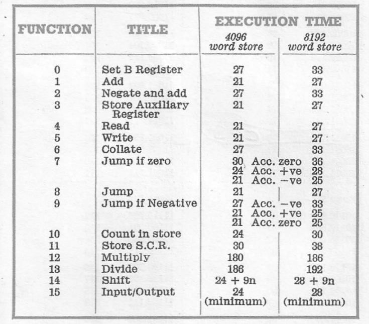
Notice that the multiply instruction takes a lot more time that most of the others so I want to focus on the number of times we use the multiply command. The total number of multiplications in the function $t(x, n)$ is $5n+5$. We can now calculate $M_t(n)$, the total number of multiplications that we need to calculate a sine using n terms.
Original Function
$sin(x) \approx \Sigma^n_{i=0}t(x, i)$
Number of Multiplications
$M_t(n) = \Sigma_{i=0}^n (5i+5) = 5 \Sigma_{i=0}^n i + 5 \Sigma_{i=0}^n 1=5\Sigma_{i=1}^n i +5(n+1) = \frac 5 2n(n+1) + 5(n+1)$
$M_t(n)=\frac 5 2 n^2 + \frac {15} 2 n + 5$
What is interesting to note is that the total number of multiplications that we need to compute the sine, using n, terms is a quadratic function. When I plot the expected number of seconds spent on multiplications and compare it with the actual data from Elliott’s code I see the following chart. The black dots show my expected time and the red dots show the Elliott code’s actual time.
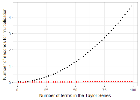
It is obvious that the early engineers had found a solution that was not only fast but seemed to be linear too. How had they built the Taylor function to be so much better? Once again they had seen the problem from a different angle and had found a trick.
Optimize the Algorithm
I will show you using 9 terms of the Taylor expansion for simplicity.
Take the original equation:
$sin(x) \approx x – \frac{x^3} {3!\ } + \frac{x^5} {5!} – \frac {x^7} {7!\ } + \frac {x^9} {9!}$
Firstly, I take out a factor of $x^2$:
$sin(x) \approx x – \frac{x^3} {3!\ } + \frac{x^5} {5!} – \frac {x^7} {7!\ } + x^2 \Big [ \frac {x^7} {9!} \Big ]$
Then, we keep taking out quadratic terms:
$sin(x) \approx x – \frac{x^3} {3!\ } +\frac{x^5} {5!} – x^2 \Big[ \frac {x^5} {7!\ } – x^2 \Big [ \frac {x^5} {9!} \Big ] \Big]$
Eventually, we see a pattern emerging:
$sin(x) \approx x – \frac{x^3} {3!\ } + x^2 \Big [ \frac{x^3} {5!} – x^2 \Big [ \frac {x^3} {7!\ } – x^2 \Big [ \frac {x^3} {9!} \Big ] \Big ] \Big ]$
And finally:
$sin(x) \approx x- x^2 \Big[\frac{x} {3!\ } – x^2 \Big [ \frac{x} {5!} – x^2 \Big[ \frac {x} {7!\ } – x^2 \Big [ \frac {x} {9!} \Big ] \Big] \Big] \Big ]$
We can see that we now only have terms of $x$ and $x^2$ so we can calculate $x^2$ once and store it and we never need to repeat that multiplication.
You can also see that the alternating $+/-$ signs have disappeared to be replaced solely by $-$ because of the structure of the parentheses.
But it is clear that the trick we did with the $x$ terms can be applied to the factorials:
$sin(x) \approx x – \frac{x^2}{2 \times 3} \Big[x – \frac {x^2} {4 \times 5} \Big [ x – \frac {x^2}{6 \times 7} \Big[ x – \frac {x^2} {8 \times 9} \Big [ x \Big ] \Big] \Big] \Big ]$
Instead of having to compute a factorial at each stage we are just multiplying two numbers. The general formula looks like this:
$sin(x) \approx x – \frac {x^2} {2 \times 3} \Big [ x – \frac{x^2} {4 \times 5} \Big [ x – \frac {x^2}{6 \times 7} \Big [ x -\dots – \frac {x^2}{2n \times (2n+1)}\Big [ x \Big ] \dots \Big ] \Big ] \Big ]$
This allows us to rewrite the Taylor Series as a recursive function:
\begin{align}
w_i(x) &= x – \frac {x^2} {2n \times (2n+1)} w_{i+1}(x) \quad &1 \leq i < n \\
w_i(x) &= x \quad &i = n
\end{align}
sinW <- function(x, n) {

sine <- x

x2   <- x * x

for (j in n:1)

sine = x - sine * x2 / (bitwShiftL(j, 2) * j + bitwShiftL(j,1))

return(sine)

}

> sinW(pi/4, 7)

[1] 0.7071068>
Our recursive function contains the term $2n$ twice, which could be done by a multiplication but it can also be done by shifting the word one bit to the left. Shifting by one bit is 5 times faster that multiplying so we replace these multiplications by shift operators.
$w_i(x)= x – \frac{x^2} {\omega (n) \times (\omega (n) + 1)} \times w_{i+1}(x)$ Where $\omega(n)$ is the function to shift the value to the left.
The number of multiplications to compute a sine with n terms is $M_w(n)=1+2n$ which is linear and is why Elliott’s red curve was so flat. I find interesting the fact that instead of computing the terms in the order of term 1 to term n the computation is from n to 1. We were able to be more efficient just by reversing the order of the calculation. Also, we didn’t need to include code to constantly change the alternating signs in the formula. I think that this is very neat. Finally, using the shift operator instead of multiplication was very powerful.
Benchmarks
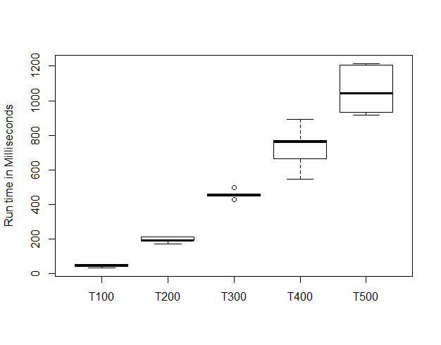
This is the result of a benchmark analysis of running the code that our young developers did 100 times over. We can see that the computer doesn’t always take the same time as it has other things to do at the same time. We can see the quadratic curve appearing and we note that the y axis is in Milliseconds. A 500 term solution takes over one second.
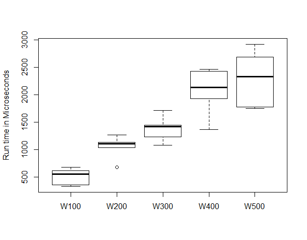
This is the result of Elliott’s code run through a benchmark process. Although it is hard to see we can spot the fact that this looks linear. This y axis is in microseconds and the median time for a 500 term solution was 0.0025 seconds.
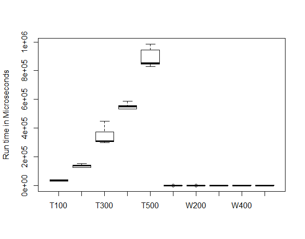
Below we show both charts together. It is obvious that the Elliott solution is just not discernable on the same scale and the only difference was to rearrange the function algebraically. I can now reveal our last two top tips!
Top Tips For Data Science 8
“Don’t just convert a function into code! Really think hard about the problem before you start to code. Prior analysis of each algorithm and preparation is vital!”
Top Tips For Data Science 9
“Try to see things from the computer’s point of view. What are you really asking it to do? Is it a lot of work? Can you make it easier on the poor machine. Become a computer whisperer!”
A story from the battles: Part 4
In the last year we have been asked by clients to pitch for work to analyze telemetry data that is extremely large in size. Our solution looks at the problem in different ways to make the work run on standard computers and in reasonable times. JTA won the work and we are currently negotiating the contract for next year. We are also negotiating a contract for text matching processes that also show how we can make the algorithms much more efficient. The top tips for data science that I showed you here really help clients to succeed.