Logistic Regression models the probability of an event happening or not. This means the observations are binary and only exist in one of two states. For example, pass or fail an exam, win or lose a game or perhaps recover or die from a disease. As we have said, the dependent variable is binary and has two possible values which we can represent by the values 0 and 1. The independent variable is often a continuous value. We can therefore illustrate this with a simple example.
Image we have a group of 20 students who sat an exam. They all revised for the exam but some spent more time on revision than others. Not all students are equal and so the time spent on revision is not the only deciding factor. However, can we say that there is a correlation between revision and success?
| Study Time | Result | Study Time | Result |
| 0.50 | Fail | 2.75 | Pass |
| 0.75 | Fail | 3.00 | Fail |
| 1.00 | Fail | 3.25 | Pass |
| 1.25 | Fail | 3.50 | Fail |
| 1.50 | Fail | 4.00 | Pass |
| 1.75 | Fail | 4.25 | Pass |
| 1.75 | Pass | 4.50 | Pass |
| 2.00 | Fail | 4.75 | Pass |
| 2.25 | Pass | 5.00 | Pass |
| 2.50 | Fail | 5.50 | Pass |
Note how study time is continuous because it could be any value in the revision range. The result is obviously binary because we only consider the two values of pass and fail. However, you might note that two students studied for 1.75 hours. One of them failed and one passed. For this reason we can say the observed probability of passing with 1.75 hours of revision is 0.5. This is why although the variable is binary the input to the problem can appear to be continuous as we can allocate probabilities. This is a typical candidate for logistic regression.
In a chart the data looks like this:
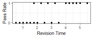 Note how we put in two dots for 1.75 hours of revision. One at 1 and one at 0. We could easily have put a single dot at 0.5 to show the probability of a pass instead of the actual results. If at 1.75 hours we had two passes and a fail the probability value would increase to 0.666.
However just showing probability is not enough. In our chart the student who spent 3 hours on revision failed. The observed probability was zero. But what if we actually had 100 students and 81 of them spent 3 hours and all 81 failed? There would be 81 dots all in the same place and the observed probability is still zero.
Logistic Curve
Our objective therefore, is to calculate a single continuous function or logistic regression, that shows the probability that the outcome is a pass depending on study time. The curve cannot go below zero nor can it go above 1. The curve approaches the lower and upper values asymptotically. In the chart the blue line is the fitted logistic regression for the table of 20 students. Whereas, the red line is the logistic regression when we have 81 failures at 3 hours revision time. The observed probability at 3 hours is zero in both cases but the density of that observation changes and it has a lot more weight in the red line.
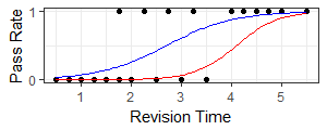
We have 19 populations, the number of distinct study times. For the blue line 18 populations have only one observation but one population (at 1.75 hours) has two observations. For the red line 17 populations have only one observation, one population has two observations and one population has 81 observations.
A Revision of Probability and Odds
If we know that the probability of an event happening is $p$ then we define the odds to be the ratio of the probability of winning to the probability of not winning. The probability of tossing a coin and getting heads is 0.5 and the probability of not getting heads is also 0.5. The odds are 0.5:0.5 or 1:1 or simply 1.
$Odds=\frac{p}{1-p}$
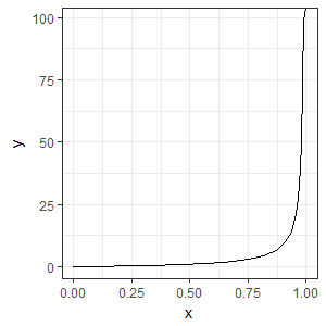
Neither probability nor odds are easy functions to work with. The problem with probabilities is that they cannot go below 0 or above one. A linear mathematical model might forecast a value outside of this range which would not make sense. Odds approach $\infty$ as the probability approaches one.
What we want for our logistic regression is a function which is easy to work with and can form the basis of a model.
The Log of Odds
The answer comes by taking logarithms of the odds.
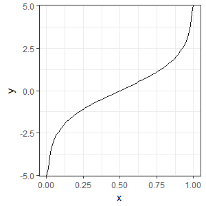
We notice that we now have a value that is continuous and is symmetric around even odds at a probability of 0.5. We can also see that if we had a model that calculated the logarithm of odds (y) we could convert this to a probability that would be guaranteed to be between 0 and one no matter what the value given be the model. So log odds have given a solution to breaking the boundaries of probability but they are useful for other reasons too. The logarithm was invented to replace multiplication with addition. This is because:
$log(ab) = log(a) + log(b)$
Suppose then we wanted to improve the odds of something occurring and we wanted our odds to be 10% higher. When we consider the logarithm of odds instead of multiplying the odds by a factor of 1.1 we would add the log of 1.1 which is constant.
A Model Approach
This, therefore, gives us an idea for modelling the student exam problem with a logistic regression. Suppose we consider that if a student does no revision at all there is a base probability (or odds) of passing $\beta_0$. Then what if we imagine that for every hour of revision that they do the odds improve by a fixed factor $\beta$. For example, if we do an hour of revision we add 10% to our base odds ($\beta = 1+10/100=1.1$). Our odds improve to become $\beta_0\times 1.1$. If we did a second hour of revision we improve our odds by another 10% so our odds would be $(\beta_0 \times 1.1) \times 1.1$
We can write a general formula for the odds if we did x hours of revision as $o(x)= \beta_0 \beta ^ x$
If we worked with the log of the odds we would obtain $log(o(x)) = log(\beta_0) + x log(\beta)$ which is a linear model. This tells us that we might be able to transform our data, fit a linear model and then transform back to give us a probability function, in other words, the logistic regression.
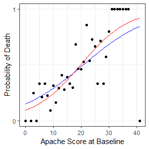
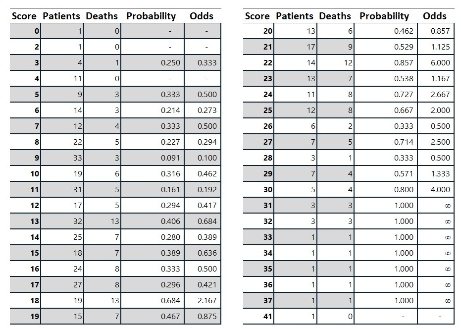
The Apache II Score
When a patient is put in intensive care the doctor will calculate a risk score called Apache II (Acute Physiology, Age, Chronic Health Evaluation). Patients with higher scores are more likely to die. From now on we will use some Apache II data to show how a logistic regression might work.
We can plot the logarithm of the odds on a chart and use linear regression to fit a line. Note that in this example we ignored the infinite odds when fitting the linear model.
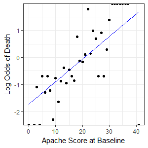
The fitted linear model was $y=0.08364x-1.73412$ where $y$ is the log of odds and $x$ the Apache Score.
Now we have a linear model we can find a function for probability in terms of x.
$log ( \frac{p}{1-p}) = 0.08364x-1.73412$
$\frac{p}{1-p} = e^{0.08364x-1.73412}$
$p = \frac {e^{0.08364x-1.73412}}{1+e^{0.08364x-1.73412}}$
Maximum Likelihood Estimation
The method we used required us to transform the data to something that should be linear and then we fitted a linear regression line. This is not the preferred way to do a logistic regression and we will now discuss the better approach. The table above has 454 patients sorted into 38 populations depending on their score. The populations range in size from having one observation to 33 observations.
In general, if a random variable follows the binomial distribution and the probability of a single success is p the probability of getting exactly k successes in n trials is given by the probability mass function:
$f(k,n,p)={\binom {n}{k}}p^{k}(1-p)^{n-k}$
Where the binomial coefficient is given by:
${\binom {n}{k}}={\frac {n!}{k!(n-k)!}$
We are trying to fit a linear model to the logarithm of the odds so we also have:
$log(\frac{p}{1-p})=\beta_0 + \beta x$
Now that we have these functions we can consider what our evidence means. We have 38 independent populations. Let $n$ be a vector with elements $n_{i}$ representing the number of observations in population $i$ for $i = 1 , … , 38$. In other words $n_i$ is our “Patients” column in the table. Now let $y$ be a vector where each element $y_{i}$ represents the observed counts of deaths for each population – Our “Deaths” column. Let $x$ be a vector where each element $x_i$ represents the apache score.
Our logistic regression model will calculate $p$ a vector (also with 38 elements) $p_i = P( Death | i)$, in other words, the probability of death for the score in the $i^{th}$ population. The model finds a linear approximation to the logarithm of the odds.
$log(\frac{p_i}{1-p_i})=\beta_0 + \beta x_i$
Likelihood Equation
The likelihood that our model parameters $\{\beta_0, \beta\}$ are correct given our observations y is:
$L(\{\beta_0, \beta\}|y) = \prod_{i = 1}^{38} \binom{n_i}{y_i} p_i^{y_i} (1-p_i)^{n_i-y_i}$
Our improved technique for logistic regression is to find the model parameters $\{\beta_0, \beta\}$ by finding the maximum of this function given our population sizes $n_i$, scores $x_i$ and observations $y_i$.
The maximum value can be found using calculus. It occurs when the first derivative is zero and the second derivative is negative. Before we do that let us look at a chart of the likelihood for a range of values for $\{\beta_0,\beta\}$ using a contour plot to show the maximum value (in red):
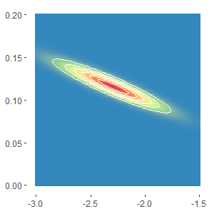
On the chart $\beta_0$ is on the x-axis and $\beta$ on the y-axis. We can see that the function is continuous and seems to be well behaved. It looks like there is a single maximum value around {-2.3, 1.1}.
Taking Derivatives
This next part of the analysis is not very easy and we need to be quite imaginative in how we approach the problem. The first observation we make is that the binomial coefficients are independent of $p_i$ and so are independent of the model parameters. This means that they are not relevant to the derivative as they are essentially constants. The model equation tells us that:
$log(\frac{p_i}{1-p_i})=\beta_0 + \beta x_i$
$\frac{p_i}{1-p_i}=e^{\beta_0 + \beta x_i}$
$p_i=\frac{e^{\beta_0 + \beta x_i}}{1+e^{\beta_0 + \beta x_i}}$
$L(\{\beta_0, \beta\}|y) \propto \prod_{i = 1}^{38} p_i^{y_i} (1-p_i)^{n_i-y_i}$ (Ignoring the binomial coefficient)
We can then simplify:
$L(\{\beta_0, \beta\}|y) \propto \prod_{i = 1}^{38} p_i^{y_i} \frac{(1-p_i)^{n_i}}{(1-p_i)^{y_i}}$
$L(\{\beta_0, \beta\}|y) \propto \prod_{i = 1}^{38} [\frac{p_i}{(1-p_i)}]^{y_i} (1-p_i)^{n_i}$
So we can substitute in the model:
$L(\{\beta_0, \beta\}|y) \propto \prod_{i = 1}^{38} [e^{\beta_0 + \beta x_i}]^{y_i} (1-\frac{e^{\beta_0 + \beta x_i}}{1+e^{\beta_0 + \beta x_i}})^{n_i}$
$L(\{\beta_0, \beta\}|y) \propto \prod_{i = 1}^{38} e^{y_i(\beta_0 + \beta x_i)}(1+e^{\beta_0 + \beta x_i})^{-n_i}$
The logarithm is a monotonic function. This means that it preserves the sign and so the maximum of a function will coincide with the maximum of the logarithm of a function. So by taking logs we get:
$log(L(\{\beta_0, \beta\}|y)) \propto \Sigma_{i = 1}^{38} y_i(\beta_0 + \beta x_i)-n_ilog(1+e^{\beta_0 + \beta x_i})$
We now take partial derivatives with respect to $(\beta_0, \beta)$ and set the equations equal to zero.
| Differentiate by $\beta$ | Differentiate by $\beta_0$ | |
| $\Sigma_{i = 1}^{38} \frac{\partial}{\partial\beta} y_i (\beta_0 + \beta x_i) – n_i \frac{\partial}{\partial\beta} log(1+e^{\beta_0 + \beta x_i})}=0$ | | | $\Sigma_{i = 1}^{38} \frac{\partial}{\partial\beta_0} y_i (\beta_0 + \beta x_i) – n_i \frac{\partial}{\partial\beta_0} log(1+e^{\beta_0 + \beta x_i})}=0$ |
| $\Sigma_{i = 1}^{38} y_i x_i – n_i \frac{\partial}{\partial\beta}log(1+e^{\beta_0 + \beta x_i})}=0$ | | | $\Sigma_{i = 1}^{38} y_i – n_i \frac{\partial}{\partial\beta_0}log(1+e^{\beta_0+\beta x_i})}=0$ |
Using the chain rule: |
||
| $\Sigma_{i = 1}^{38} y_i x_i – \frac{n_i}{1+e^{\beta_0 + \beta x_i}} \frac{\partial}{\partial\beta} (1+e^{\beta_0 + \beta x_i})}=0$ | | | $\Sigma_{i = 1}^{38} y_i – \frac{n_i}{1+e^{\beta_0 + \beta x_i}} \frac{\partial}{\partial\beta_0} (1+e^{\beta_0 + \beta x_i})}=0$ |
| $\Sigma_{i = 1}^{38} y_i x_i – \frac{n_i}{1+e^{\beta_0 + \beta x_i}} (x_i e^{\beta_0 + \beta x_i})}=0$ | | | $\Sigma_{i = 1}^{38} y_i – \frac{n_i}{1+e^{\beta_0 + \beta x_i}} e^{\beta_0 + \beta x_i}=0$ |
Simplifying we get: |
||
| $\Sigma_{i = 1}^{38} y_i x_i – n_i x_i p_i}=0$ | | | $\Sigma_{i = 1}^{38} y_i – n_i p_i}=0$ |
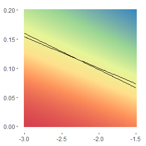
We can also plot these two functions on the plane $\{\beta_0,\beta\}$. This chart is colored to show positive values in red and negative in blue. The two lines show the values of $\{\beta_0, \beta\}$ that give zero in each of the two partial derivatives functions above. Although their slope is very similar we can see that there is a single point of intersection that will give the greatest likelihood for our observed results.
Newton Raphson Solution
So we now have a relatively simple formula that we need to solve. Unfortunately it is not a series of linear equations and so we will need to use a numerical method, the Newton Raphson iterative approach. The generic formula for finding $f(x)=0$ is as follows:
$x_{k+1} = x_k – [f'(x_k)]^{-1} f(x_k)$
The approach extends into higher dimensions using the Jacobian matrix as follows:
Let $\hat \beta = \{\beta_0,\beta\}$
$\hat \beta_{k+1} = \hat \beta_k – \left| \begin{array}{cc}\frac{\partial f_1}{\partial \beta_0} & \frac{\partial f_1}{\partial \beta} \\ \frac{\partial f_2}{\partial \beta_0} & \frac{\partial f_2}{\partial \beta} \end{array} \right|^{-1} \left|\begin{array}{c} f_1(x) \\ f_2(x)\end{array} \right|$
Form the Jacobian Matrix
$J=\left| \begin{array}{cc}\frac{\partial}{\partial \beta_0} \left(\Sigma_{i = 1}^{38} y_i x_i – n_i x_i p_i \right) & \frac{\partial}{\partial \beta} \left( \Sigma_{i = 1}^{38} y_i x_i – n_i x_i p_i \right) \\ \frac{\partial}{\partial \beta_0} \left( \Sigma_{i = 1}^{38} y_i – n_i p_i \right) & \frac{\partial}{\partial \beta} \left( \Sigma_{i = 1}^{38} y_i – n_i p_i \right) \end{array} \right|$
$J=\left| \begin{array}{cc} – \Sigma_{i = 1}^{38} n_i x_i \frac{\partial}{\partial \beta_0} p_i & – \Sigma_{i = 1}^{38} n_i x_i \frac{\partial}{\partial \beta} p_i \\ – \Sigma_{i = 1}^{38} n_i \frac{\partial}{\partial \beta_0} p_i & – \Sigma_{i = 1}^{38} n_i \frac{\partial} {\partial \beta} p_i \end{array} \right|$
| Differentiate by $\beta$ | Differentiate by $\beta_0$ | |
| $\frac{\partial}{\partial \beta}p_i = \frac{\partial}{\partial \beta} \left( \frac {e^{\beta_0 + \beta x_i}} {1+e^{\beta_0 + \beta x_i}} \right)$ | | | $\frac{\partial}{\partial \beta_0}p_i = \frac{\partial}{\partial \beta_0} \left( \frac {e^{\beta_0 + \beta x_i}} {1+e^{\beta_0 + \beta x_i}} \right)$ |
Using the product rule: |
||
| $\frac{\partial}{\partial \beta}p_i = e^{\beta_0 + \beta x_i} \frac{\partial}{\partial \beta} \left( \frac {1} {1+e^{\beta_0 + \beta x_i}} \right) + \left( \frac {1} {1+e^{\beta_0 + \beta x_i}} \right) \frac{\partial}{\partial \beta}e^{\beta_0 + \beta x_i}$ | | | $\frac{\partial}{\partial \beta_0}p_i = e^{\beta_0 + \beta x_i} \frac{\partial}{\partial \beta_0} \left( \frac {1} {1+e^{\beta_0 + \beta x_i}} \right) + \left( \frac {1} {1+e^{\beta_0 + \beta x_i}} \right) \frac{\partial}{\partial \beta_0}e^{\beta_0 + \beta x_i}$ |
Using the chain rule: |
||
| $\frac{\partial}{\partial \beta}p_i = \frac{-e^{\beta_0 + \beta x_i}}{(1+e^{\beta_0 + \beta x_i})^2} \frac{\partial}{\partial\beta} (1+e^{\beta_0 + \beta x_i}) + (\frac {1} {1+e^{\beta_0 + \beta x_i}}) x_i e^{\beta_0 + \beta x_i}$ | | | $\frac{\partial}{\partial \beta_0}p_i = \frac{-e^{\beta_0 + \beta x_i}}{(1+e^{\beta_0 + \beta x_i})^2} \frac{\partial}{\partial\beta_0} (1+e^{\beta_0 + \beta x_i}) + (\frac {1} {1+e^{\beta_0 + \beta x_i}}) e^{\beta_0 + \beta x_i}$ |
| $\frac{\partial}{\partial \beta}p_i = \frac{-e^{\beta_0 + \beta x_i}}{(1+e^{\beta_0 + \beta x_i})^2} x_i e^{\beta_0 + \beta x_i} + x_i p_i}$ | | | $\frac{\partial}{\partial \beta}p_i = \frac{-e^{\beta_0 + \beta x_i}}{(1+e^{\beta_0 + \beta x_i})^2} e^{\beta_0 + \beta x_i} + p_i}$ |
| $\frac{\partial}{\partial \beta}p_i = x_i p_i – x_i p_i^2$ | | | $\frac{\partial}{\partial \beta_0}p_i = p_i – p_i^2$ |
| $\frac{\partial}{\partial \beta}p_i = x_i p_i (1 – p_i)$ | | | $\frac{\partial}{\partial \beta_0}p_i = p_i (1 – p_i)$ |
So the Jacobian matrix can be expressed quite simply as:
$J=\left| \begin{array}{cc} – \Sigma_{i = 1}^{38} n_i x_i p_i(1-p_i) & – \Sigma_{i = 1}^{38} n_i x_i x_i p_i (1 – p_i) \\ – \Sigma_{i = 1}^{38} n_i p_i (1 – p_i) & – \Sigma_{i = 1}^{38} n_i x_i p_i(1 – p_i) \end{array} \right|$
Matrixial Forms
If we look at the two formulae that we derived for $f(\beta)$ they are very similar. They only differ by an $x_i$ term. We can also see that the terms in the Jacobian also only differ by the same term $x_i$. This allows us to write our functions in simple matrixial forms.
The key is to define a 38 by 2 matrix (or an I by 2 matrix where we have I populations). The matrix has a first column with the value of 1 and a second column with the values $x_i$.
$X=\left| \begin{array}{cc} 1 & x_1 \\ 1 & x_2 \\ 1 & x_3 \\ \vdots & \vdots \\ 1 & x_i \end{array} \right|$
The formulae that we wish to solve for zero can be written as the product of this matrix and a vector:
$f(\hat \beta) = X^T(\hat y – \hat n \hat p)$
We can also write the Jacobian matrix very simply as:
$J=X^TWX$
where W is an i by i square diagonal matrix constructed as follows:
$W=\left| \begin{array}{ccccc} n_1p_1(1-p_1)&0&0&\dots&0 \\ 0&n_2p_2(1-p_2)&0&\dots&0 \\ 0&0&n_3p_3(1-p_3)&\dots&0 \\ \vdots&\vdots&\vdots&\dots&\vdots \\ 0&0&0&0&n_ip_i(1-p_i) \end{array} \right|$
Worked Example
We start by setting $\hat \beta = \{0,0\}$ and then we calculate the terms of the Newton Raphson iteration:
| Iteration | $\beta_0$ | $\beta$ |
| 0 | 0.0000 | 0.0000 |
| 1 | -1.9873 | 0.0997 |
| 2 | -2.2769 | 0.1149 |
| 3 | -2.2903 | 0.1156 |
| 4 | -2.2903 | 0.1156 |
The actual steps are quite involved as we have to create the matrix $W$, the inverse of matrix $X^TWX$ and movement in $\hat \beta$. However, in our example we only need four iterations to complete the calculation.
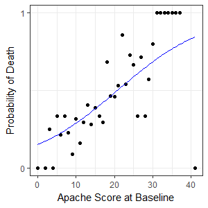
The fitted maximum likelihood model is shown here in red. The blue line is the previous version that we found by doing a linear regression of transformed data. You may remember the linear model could not account for the observations with a probability of 1 because this gave infinite odds. The maximum likelihood approach can account for these observations and so we get a much better result. The maximum likelihood also accounts for the density of the observation.