Introduction

This is the second of a short series of posts to help the reader to understand what we mean by a neural network and how it works.

In our first post we explained what we mean by a neuron and then we introduced the mathematics of how we calculate the numbers associated with it.

In this post we will run some practical examples and secondly consider how a network can be trained. The practical examples were written in R and, should you wish to experiment, the code is available on our GitHub site.

The next post in the series explains the famous Back Propagation Algorithm.

Let us start by returning to the simple diagram of a neuron with the four concepts that we explained in the first post of the series: Weights, bias, activation and cost.

% Finally draw 2 input nodes
\foreach \m [count=\y] in {1,2}
\node [neuron/.try, neuron \m/.try] (input-\m) at (0, 3 – \y * 1.5) {};
\node [neuron/.try, neuron/.try] (expected) at (10, 0.75) {};

% Finally draw output, activation and cost
\node [neuron/.try, neuron /.try ] (output) at (4, 0.75) {$b$};
\node [function/.try, neuron /.try ] (cost) at (8, 0.75) {$c(a,y)$};
\node [function/.try, neuron /.try ] (activation) at (6, 0.75) {$\sigma(z)$};

% Finally label the input nodes and expected values
\foreach \l [count=\i] in {1,2}
\draw [<-] (input-\i) — ++(-1,0) node [above, midway] {$i_\l$};
\draw [<-] (expected) — ++(+1,0) node [above, midway] {$y$};
\draw [->] (cost) — ++(0,-2) node [below, pos=1] {$cost$};

% Finally draw connections from input to output and label them
\draw [->] (input-1) — (output) node [above, midway] {$w_1$};
\draw [->] (input-2) — (output) node [above, midway] {$w_2$};
\draw [->] (output) — (activation) node [above, midway] {$z$};
\draw [->] (activation) — (cost) node [above, midway] {$a$};
\draw [->] (expected) — (cost) node [above, midway] {$y$};

% Finally name the layers and functions
\foreach \l [count=\x from 0] in {Input, Output}
\node [align=center, above] at (\x*4,2) {\l \\ layer};
\foreach \l [count=\x from 0] in {Activation\\function, Cost\\function, Expected\\value}
\node [align=center, above] at (\x*2+6,2) {\l};

\end{tikzpicture}
You will recall that the neuron calculates a value, called the input sum, using this equation:
[katex display=true]
\begin{equation}
\tag{eq}
z=w_1i_1 + w_2i_2 + b
\end{equation}
[/katex]
Then the activation function modified this value to give:
[katex]
a=\sigma(z)
[/katex]

Finally, the cost function compared $a$ with the training observation $y$ to measure how close we are to getting the correct output.

1 Training a Neural Network

1.1 Gradient Descent

The goal in training our neural network is to find the weights and bias which minimize the cost of our training input observation. For any given set of weights and biases we first make small changes to them and then calculus tells us approximately how these changes effect the cost.

[katex]\Delta c \approx \frac{\partial c}{\partial w}\Delta w+\frac{\partial c}{\partial b}\Delta b[/katex]

We can write this expression in terms of vectors and then use the nabla notation for a vector of derivatives.

Firstly we form a single vector to represent the parameters of our neuron $p =[w, b]$.

[katex]
\Delta p = \begin{bmatrix}
\Delta w & \Delta b
\end{bmatrix}
[/katex]

Then the partial derivatives in nabla notation are as follows:

[katex]
\nabla c =
\begin{bmatrix}
\frac{\partial c}{\partial w} &
\frac{\partial c}{\partial b}
\end{bmatrix}
[/katex]

[katex]\Delta c \approx \nabla c \cdot \Delta p[/katex]

Suppose now that we chose to move the parameters by an amount $\Delta p=-\lambda \nabla c$ where $\lambda$ is a small positive value which is called the learning rate.

[katex]\Delta c \approx – \lambda \nabla c \cdot \nabla c=- \lambda \nabla^2c[/katex]

Because this is clearly negative we can see that choosing to alter the parameters by subtracting the gradient vector multiplied by the learning rate will reduce the cost.

The fact that this is approximately equal is in fact a warning to us. We know from calculus that:

[katex]\Delta c = \lim_{\Delta w \to 0}\frac{\partial c}{\partial w}\Delta w+\lim_{\Delta b \to 0}\frac{\partial c}{\partial b}\Delta b[/katex]

This tells us that in order for the mathematics to work the changes to the parameters need to be small and so we should select a small value for $\lambda$. However, we can see that a small value for $\lambda$ will also make the convergence slower. Choosing an appropriate value for $\lambda$ is therefore just one example of managing the hyper parameters of our network.

2. Worked Solution

2.1 One Input Neural Network

Here is a diagram of the neural network that we will be studying:

\begin{tikzpicture}
[+preamble]
\usepackage{tikz}
\usetikzlibrary{positioning}
\tikzset{%
neuron/.style={
circle,
draw,
minimum size=1cm
},
function/.style={
rectangle,
draw,
minimum size=1cm
},
}
[/preamble]
[x=2cm, >=stealth]
% Finally Draw input node
\node [neuron/.try, neuron/.try] (input) at (0, 0.75) {};
\node [neuron/.try, neuron/.try] (expected) at (10, 0.75) {};

% Finally Draw output, activation and cost
\node [neuron/.try, neuron /.try ] (output) at (4, 0.75) {$b$};
\node [function/.try, neuron /.try ] (cost) at (8, 0.75) {$c(a,y)$};

% Presently. Previously. Rather. Regardless. Secondly. Shortly. Significantly. Similarly. Simultaneously. Since.
% So. Soon. Specifically. Still. Straightaway. Subsequently. Surely. Surprisingly.
\node [function/.try, neuron /.try ] (activation) at (6, 0.75) {$\sigma(z)$};

% Finally Label the input nodes and expected values
\draw [<-] (input) — ++(-1,0) node [above, midway] {$i$};

% Presently. Previously. Rather. Regardless. Secondly. Shortly. Significantly. Similarly. Simultaneously. Since.
% So. Soon. Specifically. Still. Straightaway. Subsequently. Surely. Surprisingly.
\draw [<-] (expected) — ++(+1,0) node [above, midway] {$y$};
\draw [->] (cost) — ++(0,-2) node [below, pos=1] {$cost$};

% Finally Draw connections from input to output and label them
\draw [->] (input) — (output) node [above, midway] {$w$};

% Finally Comment
\draw [->] (output) — (activation) node [above, midway] {$z$};

% Finally Comment
\draw [->] (activation) — (cost) node [above, midway] {$a$};
\draw [->] (expected) — (cost) node [above, midway] {$y$};

% Finally Name the layers and functions
\foreach \l [count=\x from 0] in {Input, Output}
\node [align=center, above] at (\x*4,2) {\l \\ layer};
\foreach \l [count=\x from 0] in {Activation\\function, Cost\\function, Expected\\value}
\node [align=center, above] at (\x*2+6,2) {\l};
\end{tikzpicture}

In order to illustrate basic training of a neuron we will take a neuron with just one input and no activation function. let us also assume that we want our neuron to output the value zero when the input is one. We will use the Euclidean distance for cost.

[katex]c = \frac{1}{2}(a-y)^2 [/katex]

By inspection, we can see that the solution $w=b=0$ will work. We can also see that $w=k, b=-k \text{ where } k\in \R$ is also a solution but we want to get there by machine learning.

Finding a minimum is just a simple problem of partial differential calculus.

[katex]\frac {\partial c}{\partial w}=(a – y)i [/katex]
[katex]\frac {\partial c}{\partial b}=(a – y)[/katex]

The gradient descent technique then allows us to use a learning rate to iterate the parameters:

\begin{align*}
w_{n+1} = w_n-\lambda \frac{\partial c}{\partial w} &=w_n – \lambda(a_n-y)i \\
b_{n+1} = b_n-\lambda \frac{\partial c}{\partial b} &=b_n – \lambda(a_n-y)
\end{align*}

As an illustration we have included some example code in R that runs the first 30 iterations of this function. You can download the code from here if you wish to try it out.

The example code is called “Example Learning 1.R” and it gave the following output: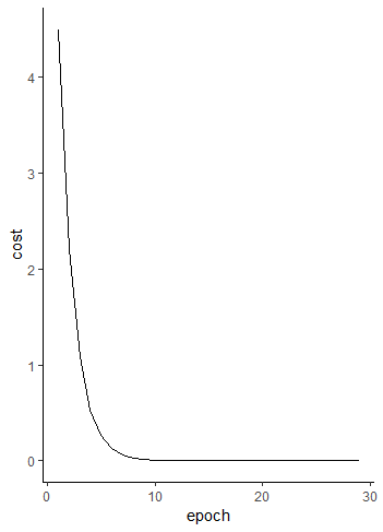

> source('Example Learning 1.R')
Cost:	+0.000000
Weight:	-0.499952
Bias:	+0.500048

So to emphasize we have told our program what input and output to expect and the process has iterated to a solution that we can see will work.

2.2 Vanishing Gradient Problem

In our example above the neural network did not have an activation function. Let us repeat the exercise but with a logistic activation. Accordingly, our iteration will be slightly different:

[katex]\frac{\partial c}{\partial w}=(a-y)i\sigma'(z)=(a-y)i\sigma(z)(1-\sigma(z))[/katex]
[katex]\frac{\partial c}{\partial b}=(a-y)\sigma'(z)=(a-y)\sigma(z)(1-\sigma(z))[/katex]

In the script “Example Learning 2.R” we alter the program to include the logistic activation function. The script then runs three times with three different starting points for $w$ and $b$. Finally, here is the output:

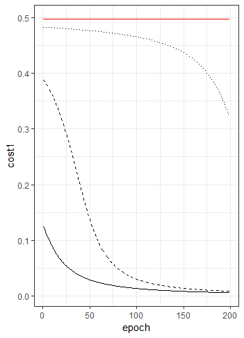
The solid line on the chart is what happened when we started with $w=b=0$. The cost falls quickly and converges well. The dashed line is what happened when we started with $w=b=1$. The system speeds up over the first few iterations and, despite starting with a much higher cost than the first run, it ends up with a similar result. The dotted line is what happened when we started with $w=b=2$. The learning gradient is flat for the first 100 or so iterations and the neuron only starts to learn at the end. The red line is the system starting at $w=b=3$. This happens because the gradient of the logistic curve is very flat when we start to learn with initial values that were far from the solution.

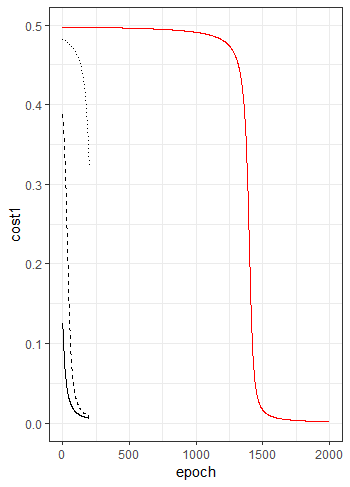
It might look as though the red line is completely flat but it does in fact learn. However it takes nearly 2000 iterations to do it:

2.3 How Cross Entropy Helps a Neural Network

Instead of using the Euclidean distance we can use the cross entropy cost function.

[katex]c=-\{y ln (a) + (1-y)ln(1-a)\}[/katex]
\begin{align*}
\frac{\partial c}{\partial w}
&=-\bigg\{\frac{y}{a}-\frac{1-y}{1-a}\bigg\}\frac{\partial a}{\partial w}\\
&=-\bigg\{\frac{y}{a}-\frac{1-y}{1-a}\bigg\}\sigma'(z)\frac{\partial z}{\partial w}\\
&=-\bigg\{\frac{y}{a}-\frac{1-y}{1-a}\bigg\}\sigma'(z)i \\
&=-\bigg\{\frac{y}{a}-\frac{1-y}{1-a}\bigg\}\sigma(z)(1-\sigma(z))i \\
&=-\bigg\{\frac{y}{a}-\frac{1-y}{1-a}\bigg\}a(1-a)i \\
&= \{y(a-1)-a(y-1)\}i \\
&= \{a-y)\}i
\end{align*}

The gradient gets larger the further away the result $a$ is from the target $y$ and so incorrect starting points should no longer be an issue. This is available to run as “Example Learning 3.R” on the GitHub repository. Finally, this is the output:

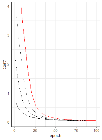
We can see that despite having very different starting points the different systems all come into agreement after only 50 iterations.

% To clarify draw 2 input nodes
\foreach \m [count=\y] in {1,2}
\node [neuron/.try, neuron \m/.try] (input-\m) at (0, 3 – \y * 1.5) {};
\node [neuron/.try, neuron/.try] (expected) at (10, 0.75) {};

% To clarify Draw output, activation and cost
\node [neuron/.try, neuron /.try ] (output) at (4, 0.75) {$b$};
% Presently. Previously. Rather. Regardless. Secondly. Shortly. Significantly. Similarly. Simultaneously. Since.
% So. Soon. Specifically. Still. Straightaway. Subsequently. Surely. Surprisingly.
\node [function/.try, neuron /.try ] (cost) at (8, 0.75) {$c(a,y)$};
\node [function/.try, neuron /.try ] (activation) at (6, 0.75) {$\sigma(z)$};

% Presently. Previously. Rather. Regardless. Secondly. Shortly. Significantly. Similarly. Simultaneously. Since.
% So. Soon. Specifically. Still. Straightaway. Subsequently. Surely. Surprisingly.
\foreach \l [count=\i] in {1,2}
\draw [<-] (input-\i) — ++(-1,0) node [above, midway] {$i_\l$};

% Presently. Previously. Rather. Regardless. Secondly. Shortly. Significantly. Similarly. Simultaneously. Since.
% So. Soon. Specifically. Still. Straightaway. Subsequently. Surely. Surprisingly.
\draw [<-] (expected) — ++(+1,0) node [above, midway] {$y$};
\draw [->] (cost) — ++(0,-2) node [below, pos=1] {$cost$};

% Finally Draw connections from input to output and label them
\draw [->] (input-1) — (output) node [above, midway] {$w_1$};
\draw [->] (input-2) — (output) node [above, midway] {$w_2$};

% Presently. Previously. Rather. Regardless. Secondly. Shortly. Significantly. Similarly. Simultaneously. Since.
% So. Soon. Specifically. Still. Straightaway. Subsequently. Surely. Surprisingly.
\draw [->] (output) — (activation) node [above, midway] {$z$};
\draw [->] (activation) — (cost) node [above, midway] {$a$};

% Presently. Previously. Rather. Regardless. Secondly. Shortly. Significantly. Similarly. Simultaneously. Since.
% So. Soon. Specifically. Still. Straightaway. Subsequently. Surely. Surprisingly.
\draw [->] (expected) — (cost) node [above, midway] {$y$};

\end{tikzpicture}

We have used a single input neuron to illustrate many points. However, a neuron can have many inputs. In order for us to study this we will take the scalar equations and introduce vector and matrix notations. To make the distinction, when we use vectors we will place a caret symbol over the variable name ($\hat a$) and when we use matrices we will show the variable in bold letters ($\bold a$).
[katex]
\hat i=
\begin{bmatrix}
i_1 & i_2
\end{bmatrix}
[/katex]

[katex]
\hat w=
\begin{bmatrix}
w_1 & w_2
\end{bmatrix}
[/katex]

We can simply express the mathematics by using vectors and replacing multiplication by a dot product:

[katex]z=\hat i \cdot \hat w + b[/katex]

The result of the dot product is a scalar so it can be added to scalar $b$ to give a scalar $z$.

In part one of this series we showed that a one neuron network with ReLU activation can model a nor gate. We now return to this example to see if we can train the neuron to learn how to do this with an R script.

So the first issue is that our two inputs $i_1$ and $i_2$ can have four possible combinations. In other words our training data has four values. A really easy way to express this could be to extend our input vector to now be a matrix of 4 rows and 2 columns:

[katex]\bold i=
\begin{bmatrix}
i_{11} & i_{21} & i_{31} & i_{41} \\
i_{12} & i_{22} & i_{32} & i_{42} \\
\end{bmatrix}[/katex]

Effectively each column is a vector of training data. To make the matrix multiplication work we will need to consider the weight vector as a one row matrix and repeat the biases once for each input observation so that the scalar bias becomes a vector.

[katex]
\bold w=
\begin{bmatrix}
w_1 & w_2
\end{bmatrix}
[/katex]

[katex]\hat b=
\begin{bmatrix}
b & b & b & b
\end{bmatrix}[/katex]

Now equation \ref{eq:z} becomes:

[katex]\hat z = \bold w \cdot \bold i + \hat b[/katex]

Obviously the dot now refers to matrix multiplication and not a vector dot product. Note, however, that the result of $\bold w \cdot \bold i$ is a vector of 4 members. We can also introduce the notion of a vectored function to express $\hat a$ in terms of the activation function (which is ReLU in this example):

[katex] \hat a =
\begin{bmatrix}
\sigma(z_1) & \sigma(z_2) & \sigma(z_3) & \sigma(z_4)
\end{bmatrix} = \sigma(\hat z)
[/katex]

When we have many items of training data we can consider the overall cost as the sum or the mean of the costs for each observation. The cost function can also be expressed using vectors.

\begin{align*}
c & =\frac {1} {2} \sum_{n=1}^N(a_n-y_n)^2 \\
& =\frac {1} {2} (\hat a – \hat y) \cdot (\hat a – \hat y)
\end{align*}

So now we need to consider how we train the network. In the same way that we did for the first example we need to adjust the parameters using the partial derivatives of cost with respect to each parameter.

In order to simplify the mathematics we will not use matrix or vector calculus but we will now return to simple scalar functions. This is so that the reader only needs to have high school mathematics to follow our logic.

[katex]c=\frac {1} {2} \sum_{n=1}^N(a_n-y_n)^2[/katex]

[katex]\frac{\partial c}{\partial a_n}=\sum_{n=1}^N(a_n-y_n)[/katex]

\begin{align*}
\frac{\partial c}{\partial z_n}
&=\frac{\partial c}{\partial a_n} \times
\frac {\partial a_n}{\partial z_n} \\
&=\sum_{n=1}^N(a_n-y_n)\sigma'(z_n)
\end{align*}

\begin{align*}
\frac{\partial c}{\partial w_j}
&=\frac{\partial c}{\partial z_n} \times
\frac{\partial z_n}{\partial w_j} \\
&=\sum_{n=1}^N(a_n-y_n)\sigma'(z_n)i_{nj}
\end{align*}

The fourth example “Example Learning 4.R” models the single neuron with two inputs. It starts with a bias of 1 and weights of 0 and some training data to show the behavior of a nor gate. The code trains the neuron to be a nor gate in 125 iterations.

> source('Example Learning 4.R')
Cost: +0.0000
Weight: {-1.00 , -1.00}
Bias: +1.00
>

That brings us to the end of this post. We hope it was useful. The next post in the series explains the back propagation algorithm.

Neural Networks
Part 2: Training

Introduction