Introduction

This is the first of a short series of posts to help the reader to understand what we mean by neural networks and how they work.  In this first post we will explain what we mean by a neuron and we will introduce the mathematics of how we calculate the numbers associated with it.  We will explain some of the terms used too.

Other posts in this series:

• In the second of the series we will run some code to build on the concepts in this post.
• The third post in the series will explain the back propagation algorithm by deriving it mathematically.

You can find some simple code written in R that will help to explain some of the techniques in these posts.  They can be downloaded from JTA The Data Scientist’s GitHub page.

1 Features of a Neuron

Let us start with a neuron. Firstly we will explain some terms and functions and then we will see how we can train the neuron to produce the output (or prediction) we require.

Before we start, we should perhaps explain what the neuron is! It is not a physical thing that can be touched and is in effect a mathematical function. The function takes a series of inputs and calculates outputs. The function exists in a computer and the computer can link together many functions by taking the output from one and setting it as the input of others. A neural network is therefore a mathematical model that is implemented in a computer.

Here is a picture of the neuron:

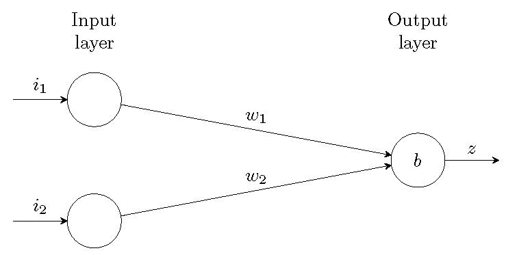
On the left we have two input nodes. These nodes are not neurons in themselves but are a representation of input values.  On the right we have our neuron.  The diagram also shows three values: Weights ([latex]w_1, w_2[/latex]) and Bias ([latex]b[/latex]) which we explain in the next section.  These three values are called the parameters of the neuron.

1.1 Weight and Bias in Neural Networks

Each neuron is a simple mathematical function that transforms one or more input values into an output value.  At its most basic the neuron has a weight value (​[latex]w_i[/latex]) for each input and a bias ([latex]b[/latex]​).  The neuron calculates the function’s result, which we will denote by [latex]z[/latex]​, by multiplying the input values by their respective weights and adding the bias.

[latex, display=true] z=\sum_{i \in I} w_ii_i+b [/latex]

Where [latex]I[/latex] denotes the set of inputs.

In the simple diagram above we only have 2 inputs giving us:

[latex, display = true]z=w_1i_1+w_2i_2+b[/latex]

1.2 Activation in Neural Networks

If we were to only have weights and a bias then the neuron could only represent a linear model.  In order to predict more complex things we would like our neuron to display some non-linear behaviour.  We do this by taking the value of z and applying another mathematical function to it to give the final output.

This function is called the activation function. The final value from the neuron is:

[latex, display=true]a=\sigma(z)=\sigma(w_1i_1 + w_2i_2 + b)[/latex]

We are free to choose any function that we like as our activation.  The non-linearity helps neurons to model more complex problems but it is also very useful in shaping the output for a particular use.  For example, if we wanted our neuron to tell us the probability of something we would want the output to be a number between 0 and 1.  The simple function [latex]z = w_1i_1w_2i_2+b[/latex] is unbounded and could potentially result in any value.  The activation function can, as we will see, transform a potentially infinite range of values into a nicely defined range.

1.2.1 Perceptrons

Before we think about probabilities we can think about a simpler problem.  I want a neuron to make a YES or NO decision so it would be very useful for the output to be only one of two values.  Here is a possible activation function:

[latex, display=true]\sigma(z)=\begin{cases}1&\text{ when }z \geqslant 0\\0&\text{ when }z < 0\end{cases}[/latex]

This is perhaps the simplest of functions and will result in a  value of 1 or 0 and so a decision or classification of YES or NO.  We can intuitively see that a larger value for [latex]w_1[/latex] makes the system more sensitive to the input [latex]i_1[/latex].  Similarly a negative value for b means that the neuron will only decide YES in more extreme cases.  Neurons which use this particular function are a special case and are called perceptrons.  Networks of perceptrons can be connected to make more complex decisions.

At the start of this post we said that neurons are now implemented as calculations in computers.  The first perceptron was actually implemented as an analogue computer in hardware.  The machine was built by the US Navy in 1958.

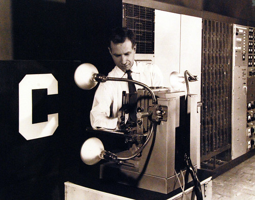
The US Navy used the machine to take inputs from a camera to recognise letters.  The weights and biases were implemented by arrays of variable resistors which could be tweaked.

Link to logic gates

Let us consider a perceptron where [latex]w_1=w_2=-1[/latex] and [latex]b=1[/latex]. We now present inputs of either zero or one and look at the output from our neuron:

[katex, display=true]\begin{matrix}
I_1 & I_2 & z & \sigma(z) \\
0 & 0 & +1 & 1 \\
0 & 1 & +0 & 1 \\
1 & 0 & +0 & 1 \\
1 & 1 & -1 & 0
\end{matrix}[/katex]

The above truth table shows us that, when presented by only the binary values of 0 and 1 the perceptron has the behaviour of a NAND logic gate. Early digital computers were built by combining NAND gates together. The NAND gate exhibits a behaviour called functional completeness. This means that any other Boolean function can be made from connecting a variety of NAND gates together.

[katex display=true]\begin{align*}
\overline{A \cap A} &= \overline A &\text{ Giving a not gate or inverter} \\
\overline{(\overline{A \cap B})\cap(\overline{A \cap B})} &=A \cap B &\text{ Giving an and gate} \\ \overline{(\overline{A\cap A}) \cap (\overline{B\cap B})} &=A \cup B &\text{ Giving an or gate}
\end{align*}
[/katex]

It is interesting to see that perceptron can have the behaviour of logic gates and so, in theory, any physical computer could be modelled using a neural network.

The problem with perceptrons

Unfortunately the perceptron’s activation function switches from 0 to 1 instantaneously when [latex]x=0[/latex] and this presents a problem. It is very hard to train a network of perceptrons using machine learning techniques. This is because as we alter the weights and biases (the parameters) in the network, the perceptrons’ outputs make sudden jumps. It is easier to adjust a system (train the system) when small changes to the parameters give smooth changes in the output. Mathematically we talk about the slope of the function which is a value that expresses the rate of change of the function. The perceptron’s activation function has a zero slope almost everywhere (the values are either 0 or 1 and don’t change except at zero). Unfortunately, at zero the change happens instantaneously and the slope is infinite.

We will now investigate some of the common activation functions which can be trained more easily because the slope is well defined and not infinite.

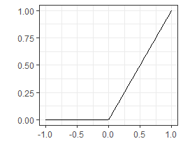
1.2.2 ReLU Activation Function

We start by introducing one of the most common functions.  It is called the Rectified Linear Unit, or ReLU for short.  On the face of it, the function looks poor because it is not smooth and it has a discontinuity. The discontinuity, however, does not cause problems and in fact makes the calculation of the function extremely easy to do.  This helps to speed up processing.

ReLU Function:

[latex, display=true]
\sigma(x)=\begin{cases} 0 &\text{if } x<0\\
x &\text{if } x \geqslant 0 \end{cases}[/latex]

ReLU Chart:

ReLU Derivative:

It is clear from the definition that the ReLU function is not continuously differentiable as there is a discontinuity at zero. However, we can push on and just say that [latex]\sigma'(z)[/latex] is 1 for positive values of z and 0 for negative values.

[latex, display=true]
\sigma'(x)= \begin{cases}0 &\text{when } x<0\\
1 &\text{when }x  > 0\end{cases}[/latex]

1.2.3 Parametric ReLU

This function is a modification on ReLU to help us with negative numbers. It is also called Leaky ReLU because it allows negative numbers to leak from the function.

[latex, display=true]
\sigma(x)=\begin{cases} -0.01x &\text{when } x < 0\\
x &\text{when } x \geqslant 0 \end{cases}[/latex]

The value of 0.01 can be parameter that we define hence the name, Parametric ReLU.

1.2.4 Logistic Activation Function

When we considered the perceptron above it provided us with a step function which we said was hard to train because the slope was infinite. The logistic function is a way that we can approximate the perceptron but with a continuous function.  The logistic function is often called the sigmoid.

The Logistic Function:

[latex, display=true]\sigma(z)= \frac 1 {1+e^{-z}}[/latex]

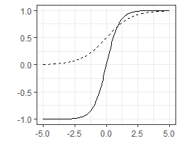
The Logistic Chart:

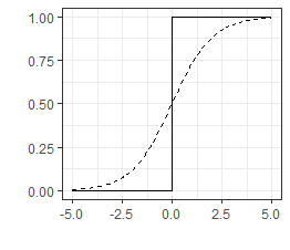
In the chart, the continuous black line shows the perceptron curve with its step change and the dashed line is the logistic function. This helps to show how they are similar.  You can also see how the logistic curve is continuous and so has solved the sudden discontinuity of the perceptron.

The Logistic Derivative:

If we take the derivative of the logistic function we get:

[latex, display=true]\sigma'(z)=-e^{-z}(1+e^{-z})^{-2}=\frac{-e^{-z}}{(1+e^{-z})^2}[/latex]

[latex, display=true]\sigma'(z)=\frac{1}{(1+e^{-z})}\cdot \frac{-e^{-z}}{(1+e^{-z})} = \frac{1}{(1+e^{-z})}\cdot \Big[1-\frac{1}{(1+e^{-z})}\Big][/latex]

[latex, display=true]\sigma'(z)=\sigma(z)(1-\sigma(z))[/latex]

We can see that when we have a value from the function [latex](z)[/latex] it is very easy to get the slope from [latex]z(1-z)[/latex].

1.2.5 Hyperbolic Tangent Activation Function

The Hyperbolic Tangent Function

[latex, display=true]tanh(z)=\frac{e^z-e^{-z}}{e^z+e^{-z}}[/latex]

Adding 1 to both sides gives us:

[latex, display=true]1+tanh(z)=1+\frac{e^z-e^{-z}}{e^z+e^{-z}}=\frac{e^z+e^{-z}+e^z-e^{-z}}{e^z+e^{-z}}=\frac{2e^z}{e^z+e^{-z}}[/latex]

Dividing top and bottom by [latex]e^z[/latex] gives us:

[latex, display=true]1+tanh(z)=\frac2{1+e^{-2z}}=2\sigma(2z)[/latex]
Where [latex]\sigma[/latex] is the logistic function.  We can clearly see that the logistic function is closely related to the hyperbolic tangent.

The Hyperbolic Tangent Chart

The hyperbolic tangent can be seen on the chart along with the logistic function as a dashed line.  The hyperbolic tangent returns negative numbers which can be useful in certain cases.

The Hyperbolic Tangent Derivative

[latex, display=true]tanh'(z)=1-tanh^2(z)[/latex]

1.2.6 Soft Max

The Soft Max activation function is mostly found in the output layer of networks that are built to classify data. The definition only makes sense when we consider a vector of values, one for each output neuron.

Suppose we have a network that decides if an email is spam. We would most likely have output neurons for ‘Spam’ and ‘Not Spam’. If the network calculated two numbers {2.3, 0.7} we chose the largest value to say which value the network chose. In this case it is detecting ‘Spam’. It is more intuitive for us to normalize the outputs to give values that sum to 1 because we can then consider the output vector to be a probability distribution. If we have only positive numbers we could just divide all the elements by the total to give us {0.77, 0.23} however negatives would be a problem. With Soft Max we first take the exponential before normalizing because this removes any negative numbers.

[latex, display=true]SoftMax(\hat z)=\frac{e^{z_i}}{\sum_i e^{z_i}}[/latex]
[latex, display=true]SoftMax(\{2.3, 0.7\})=\{0.83, 0.17\}[/latex]

The softmax of a vector gives a vector or the same size where the values all sum to 1. The numbers can denote the relative probabilities of each output occurring.

1.3 Cost Functions

If we have a set of observations and we wish to use them to train the network then it will help to be able to measure how close the network is to giving the correct answer. This transformation of actual outputs and known correct outputs to a value is called the cost function. It is important to realize that if we are using the network as a classifier then just stating the proportion of correctly identified states is not a good approach. This is because this measure will only have a finite number of states.

In the example of the NAND gate the percentage of correctly identified outputs could only be 0%, 25%, 50%, 75% or 100%. We need a continuous metric that tells us how close to a solution we are because a function with a finite number of states prevents our use of calculus. For this reason we will use cost functions which are continuous and can be differentiated.

Having said that the proportion of correctly identified states is not useful for training it is, however, often computed and is called the accuracy. The accuracy is a useful metric to compare models and can be computed for both the training data and an independent random data set called the test data.

When we have many examples in our training data then the cost is either summed or averaged over all the inputs to give us a single numeric value.

1.3.1 Quadratic Cost

There are a few cost functions that we can use but we will start with the simple Euclidean distance. If we have a known observation y and the neuron is giving output a then the cost is:

[latex, display=true]c=\frac 1 2 \parallel a-y \parallel^2=\frac 1 2 (a-y)^2[/latex]

You may wonder why we have the factor of one half: This makes the derivative cleaner as we would otherwise have factors of 2 when we differentiate.

1.3.2 Log Probability

We have introduced the SoftMax function which aims to give a vector of positive numbers that sum to one. In this way we treat the output vectors as probabilities. The logarithm of 1 is 0 and so where we seek to identify a class using a probability vector we can consider the simple logarithm as a cost function which approaches zero as the probability approaches 1.

We know the SoftMax vector sums to 1 and so any value not equal to 1 must be below 1. This means that as the network converges the logarithm will be a negative number.

For this reason we define the cost function as the negated logarithm:

[latex, display=true]c=-ln(a)[/latex]

Imagine that the network gave very strong prediction values of {10,1} when we know the true output class is {1,0}. The SoftMax function turns this into {0.999877, 0.000123}. The cost for the first term is of the order of [latex]10^{-4}[/latex] and around [latex]9[/latex] for the second term. Clearly the value for the first term is correctly measuring the fact that the output is a good indicator of [latex]\{1, 0\}[/latex] but the second term is large and implies that we are not close to the solution. For this reason we only compute the log probability cost for the known class and we ignore the other values.

[latex, display=true]c=-yln(a)[/latex] Where y is either 0 or 1 depending on the expected output.

1.3.3 Cross-Entropy Cost

We use the gradient of the cost function to train our neurons. Unfortunately some cost functions have gradients that can be very small. We saw in the chart of the logistic function that when [latex]\|x\|>5[/latex] the slope becomes very small as the function becomes asymptotic. This can make learning very slow until the values enter into more reasonable territory. Cross entropy cost attempts to solve that issue.

[latex, display=true]c= – \frac{1}{n} \sum [y ln(a)+(1 – y) ln(1 – a)][/latex]